%load_ext autoreload
%autoreload 2

Two Dimensional models

Models

1. Diffusion

2. Convection

3. Convection Diffusion

All models calculated using the finite-difference method in 2 dimensions.

The models can be visualised using two types of animations.

1. Color animated plots

2. 3D animated plots

These partial differential equations are solved for a function \(u(x, t)\) in discretized time \(t\) and space \(x\). See source code diffuconpy to see the full implementation of the finite difference method.

import numpy as np
import matplotlib.pyplot as plt
plt.style.use("dark_background")
import sys, os

sys.path.append(os.path.abspath(os.path.join('..')))

import diffuconpy as dc
import animations

class ExamplePlot:
    
    def __init__(self, model, dx, title, limx, limy, fps, frn, filename):
        self.model = model
        self.title = title
        self.limx = limx
        self.limy = limy
        self.fps = fps
        self.frn = frn
        self.filename = filename
        self.dx = dx

        xvar = np.arange(limx[0], limx[1], self.dx)
        yvar = np.arange(limy[0], limy[1], self.dx)

        self.X, self.Y = np.meshgrid(xvar, yvar)

        

    def CreateAnimation_color(self):
        """
        Saves a colour plot animation as a GIF file. 2 dimensional solutions only.
        """
        try:   
            animations.animation_color(solution=self.model.solution, xlab='x', ylab='y', title=self.title, xlim_=self.limx, ylim_=self.limy, fps=self.fps, frn=self.frn, filename=self.filename)
            print('PLOT SAVED SUCCESSFULLY \n--------------------')
        except:
            Exception('ERROR!')

    def CreateAnimation_3D(self):
        """
        Saves a 3D plot animation as a GIF file. 2 dimensional solutions only.
        """
        try:   
            animations.animation_2(solution=self.model.solution, X=self.X, Y=self.Y, xlab='x', ylab='y', zlab='solution', title=self.title, zlim=(-5, 10), fps=self.fps, frn=self.frn, filename=self.filename)
            print('PLOT SAVED SUCCESSFULLY \n--------------------')
        except:
            Exception('ERROR!')

# Initialising the models.
# All models shown here will use all these same parameters
dx = 0.1
dt = 0.1
limx = (-5, 5)
limy = (-5, 5)
fps = 60
frn = 250

xvar = np.arange(limx[0], limx[1], dx)
yvar = np.arange(limy[0], limy[1], dx)

X, Y = np.meshgrid(xvar, yvar)

init = 4*(1/np.sqrt(0.01*2*np.pi))*np.exp(-(1/2)*((X**2 + Y**2)/0.1))

Diffusion and convection coefficents

see Convection Diffusion.

diffusion = 0.009
convection = -0.1

Boundary Conditions

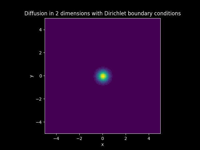
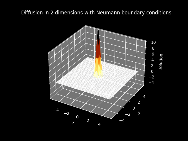
In the models that have diffusion, boundary conditions are imposed. The boundary of the solution is set to zero everywhere when Dirichlet boundary conditions are imposed. The boundary of the flux or the first derivative of the solution is set to zero everywhere when Neumann boundary conditions are imposed.

boundary = [0, 0, 0, 0]
flux_boundary = [0, 0, 0, 0]

Diffusion

Color plots

Nt1 = 250
Nx1 = 100

TITLE_1_D = 'Diffusion in 2 dimensions with Dirichlet boundary conditions'
FILE_1_D_color = 'img//animation_diffusion_2dims_dirichlet_color.gif'

TITLE_1_N = 'Diffusion in 2 dimensions with Neumann boundary conditions'
FILE_1_N_color = 'img//animation_diffusion_2dims_neumann_color.gif'

model1 = dc.diffusion_2dims(Nt1, Nx1, dt, dx, diffusion, init)

# Dirichlet boundary conditions
sol1_dirichlet = model1.solve_Dirichlet(boundary)

# Neumann boundary conditions 
sol1_neumann = model1.solve_Neumann(flux_boundary)


model1_plot_D = ExamplePlot(sol1_dirichlet, dx, TITLE_1_D, limx, limy, fps, frn, FILE_1_D_color)

model1_plot_N = ExamplePlot(sol1_neumann, dx, TITLE_1_N, limx, limy, fps, frn, FILE_1_N_color)

model1_plot_D.CreateAnimation_color()
model1_plot_N.CreateAnimation_color()

PLOT SAVED SUCCESSFULLY 
--------------------

PLOT SAVED SUCCESSFULLY 
--------------------

Animations

3D plots

FILE_1_D_3D = 'img//animation_diffusion_2dims_dirichlet_3D.gif'
FILE_1_N_3D = 'img//animation_diffusion_2dims_neumann_3D.gif'

model1_plot_D = ExamplePlot(sol1_dirichlet, dx, TITLE_1_D, limx, limy, fps, frn, FILE_1_D_3D)
model1_plot_N = ExamplePlot(sol1_neumann, dx, TITLE_1_N, limx, limy, fps, frn, FILE_1_N_3D)

model1_plot_D.CreateAnimation_3D()
model1_plot_N.CreateAnimation_3D()

Animations

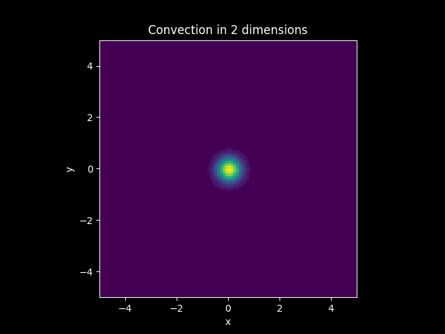
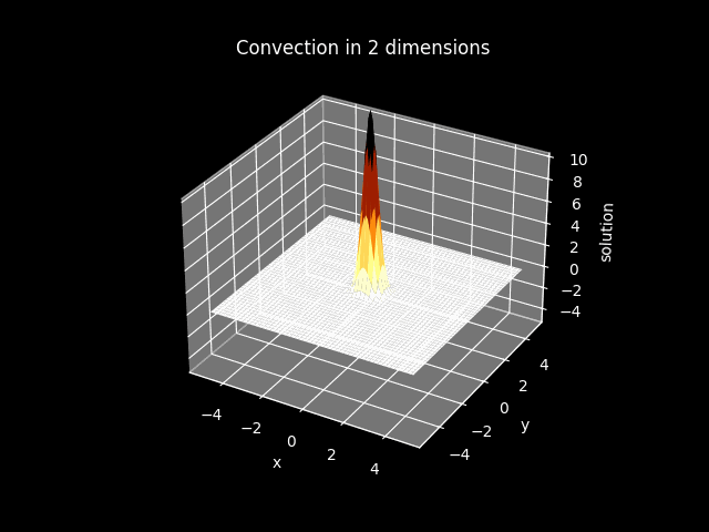
Convection

Color plots

Nt2 = 250
Nx2 = 200

TITLE_2 = 'Convection in 2 dimensions'
FILE_2_color = 'img//animation_convection_2dims_color.gif'

model2 = dc.convection_2dims(Nt2, Nx2, dt, dx, convection, init)

sol2 = model2.solve()

model2_plot = ExamplePlot(sol2, dx, TITLE_2, limx, limy, fps, frn, FILE_2_color)

model2_plot.CreateAnimation_color()

PLOT SAVED SUCCESSFULLY 
--------------------

Animations

3D plots

FILE_2_3D = 'img//animation_convection_2dims_3D.gif'

model2_plot = ExamplePlot(sol2, dx, TITLE_2, limx, limy, fps, frn, FILE_2_3D)

model2_plot.CreateAnimation_3D()

PLOT SAVED SUCCESSFULLY 
--------------------

Animations

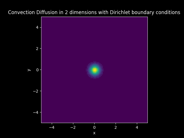
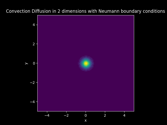
Convection Diffusion

Color plots

Nt3 = 250
Nx3 = 200

TITLE_3_D = 'Convection Diffusion in 2 dimensions with Dirichlet boundary conditions'
FILE_3_D_color = 'img//animation_convection_diffusion_2dims_dirichlet_color.gif'

TITLE_3_N = 'Convection Diffusion in 2 dimensions with Neumann boundary conditions'
FILE_3_N_color = 'img//animation_convection_diffusion_2dims_neumann_color.gif'

model3 = dc.convection_diffusion_2dims(Nt3, Nx3, dt, dx, diffusion, convection, init)

# Dirichlet boundary conditions
sol3_dirichlet = model3.solve_Dirichlet(boundary)

# Neumann boundary conditions 
sol3_neumann = model3.solve_Neumann(flux_boundary)


model3_plot_D = ExamplePlot(sol3_dirichlet, dx, TITLE_3_D, limx, limy, fps, frn, FILE_3_D_color)

model3_plot_N = ExamplePlot(sol3_neumann, dx, TITLE_3_N, limx, limy, fps, frn, FILE_3_N_color)

model3_plot_D.CreateAnimation_color()
model3_plot_N.CreateAnimation_color()

PLOT SAVED SUCCESSFULLY 
--------------------
PLOT SAVED SUCCESSFULLY 
--------------------

Animations

3D plots

FILE_3_D_3D = 'img//animation_convection_diffusion_2dims_dirichlet_3D.gif'
FILE_3_N_3D = 'img//animation_convection_diffusion_2dims_neumann_3D.gif'

model3_plot_D = ExamplePlot(sol3_dirichlet, dx, TITLE_3_D, limx, limy, fps, frn, FILE_3_D_3D)
model3_plot_N = ExamplePlot(sol3_neumann, dx, TITLE_3_N, limx, limy, fps, frn, FILE_3_N_3D)

model3_plot_D.CreateAnimation_3D()
model3_plot_N.CreateAnimation_3D()

PLOT SAVED SUCCESSFULLY 
--------------------
PLOT SAVED SUCCESSFULLY 
--------------------

Animations

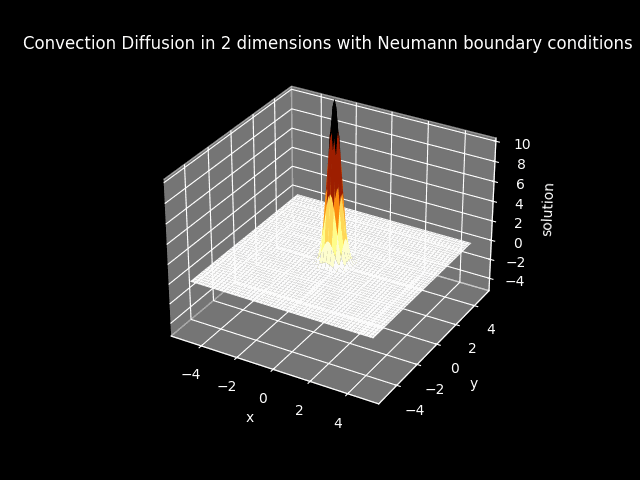
Warning: The 3D animation are extremely slow to generate, with at most 1 minute run time.

It is better to generate these solutions as color plot animations, with at most 11 seconds run time.