%load_ext autoreload
%autoreload 2
One Dimensional Transport equation#
import numpy as np
import matplotlib.pyplot as plt
import matplotlib.animation as animation
plt.style.use("dark_background")
import sys, os

sys.path.append(os.path.abspath(os.path.join('..')))

import diffuconpy as dc
import animations
The One dimensional Convection (Advection) Model, or Transport equation, is governed by the following pde:
Which initial condition:
Solving this model numerically one would have to discretize this model. One such discretization is the “Upwind Method” or “Centered difference”.
See source code diffuconpy to see the full implementation of this discretization.
To model the Advection Equation, one must consider the number of step the model will advance in time Nt = 250 and space Nx = 1500. Also \(\Delta t\) which is dt = 1/Nt in the code below and \(\Delta x\) which is dx = (5-(-5)/Nx). the boundary points on this plot are \(-5\) and \(5\), at which the initial function is \(0\). the Convection coefficient convection is \(0.75\).
# Numbers of space and time steps
Nt = 900
Nx = 1500

# Space and time step size
dt = (2-0)/Nt
dx = (5-(-5))/Nx

# Convection Coefficient (speed of the distribution)
convection = 0.75

# Setting up the initial condition
x = np.arange(-5, 5, dx)

# Initial Array
init = 3*np.sin(((2*np.pi)/5)*x)
Solving the PDE and Calculating its CLF value#
# Solving the diffusion equation
def solve(Nt, Nx, dt, dx, convection, init):
    transport = dc.convection_1dims(Nt, Nx, dt, dx, convection, init)
    model = transport.solve()

    return model.solution
density = solve(Nt, Nx, dt, dx, convection, init)

CLF = np.abs(convection*(dt/dx))

print(CLF)
0.25
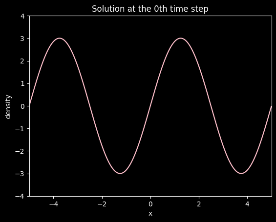
Plotting the first time step#
# Plotting the 0th time step state
plt.figure(0)
ax = plt.axes(xlim=(-5, 5), ylim=(-4, 4)) # left bound -5 and right bound 5
ax.plot(x, density[0], color='pink')
plt.title('Solution at the 0th time step')
plt.xlabel('x')
plt.ylabel('density')
plt.show()
Animating the Solution#
# Setting up the animation
FPS = 60
FRN = 250
FILE = './img/convection_in_1_dimension.gif'

# Calling the animation_() function defined in the previous cell.
# See the animation at ./example-img/convection_in_1_dimension.gif
animations.animation_1(
    solution=density,
    X=x,
    xlab='x',
    ylab='density',
    title='Solution to Transport Equation',
    color='pink',
    xlim_=(-5, 5),
    ylim_=(-4, 4),
    fps=FPS,
    frn=FRN,
    filename=FILE
    )
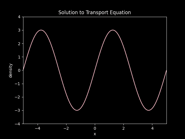
Convection of a sinwave at a speed of 0.75.