Challenger Disaster: O-Rings and Logistic Regression

On January 28th, 1986, the Space Shuttle Challenger lifted off from Cape Canaveral, Florida. 73 seconds later 14km off the ground, it desintegrated killing all of its crew including the school teacher Christa McAuliffe.

The cause of failure was primary and secondary O-ring seals in the right Space Shuttle Solid Rocket Booster. The record low morning temperatures of $36^\circ$ Fahrenheit ($2^\circ$ Celsius) caused the rubber O-rings to stiffen up and loose their ability to seal the joints on the Boosters.

Below is footage of the launch from NBC News on YouTube.

In this post we will investigate the probability of an O-ring failing with respect to the air tempurature around the launch site, using Logistic Regression.

The Challenger O-ring data was found at the University of California, UC Irvine Machine Learning Repository.

Firstly we need to download the dataset. We can use the GET function in the httr library in R to fetch the data and unpack it with the zip function. To insall these libraries run the following in the R terminal

install.packages("httr")
install.packages("zip")
install.packages("gmodels")

Then.

library(httr)
library(zip)
library(ggplot2)

Next we will download the data.

# Define the URL and the output file path
url <- "https://archive.ics.uci.edu/static/public/92/challenger+usa+space+shuttle+o+ring.zip"
output_zip <- "challenger_usa_space_shuttle_o_ring.zip"
output_dir <- "challenger_usa_data"

# Download the ZIP file
cat("Downloading the dataset...\n")
GET(url, write_disk(output_zip, overwrite = TRUE))

# Create a directory to extract the data
if (!dir.exists(output_dir)) {
  dir.create(output_dir)
}

# Unzip the file
cat("Extracting the dataset...\n")
unzip(output_zip, exdir = output_dir)
extracted_files <- list.files(output_dir, recursive = TRUE)
cat("Extracted files:\n")
print(extracted_files)

file.remove(output_zip)

cat("Data has been downloaded and extracted to:", output_dir, "\n")

Now we must read the data into R and save it as a dataframe to perform regression analysis on it. We will also assign column names to the dataframe to make it easier to work with.

# Specify the path to your data file
file_path <- "challenger_usa_data/o-ring-erosion-or-blowby.data"

# Load the data
df <- read.table(file_path, header = FALSE)

colnames(df) <- c(
    "num_O_rings",
    "num_failure",
    "launch_temp",
    "leak_check_pressure",
    "temporal_order"
    )

print(head(df))

num_O_rings num_failure launch_temp leak_check_pressure temporal_order
1           6           0          66                  50              1
2           6           1          70                  50              2
3           6           0          69                  50              3
4           6           0          68                  50              4
5           6           0          67                  50              5
6           6           0          72                  50              6

The column num_failure is the number of O-ring failures on a given launch. We are only interested in whether of not atleast one O-ring failed during a launch. Therefore, consider $y_i$ be a bernoulli random variable such that,

We will create a new column in df called if_failure which will describe $y_i$. Using the ifelse function in R enables us to do this.

df$if_failure <- ifelse(df$num_failure > 0, 1, 0)

The regression will be set up in the following way, let

1. Response: The probability of at least one O-ring failing $p_i$
2. Predictor: The air temperature around the launch pad $x_{temp, i}$.

Since the response is a probability, it does not make sense to use a standard linear regression. We need to use a transformation that is bounded between 0 and 1. The best choice of transformation is the Sigmoid or logistic transformation, written as

where $\eta_i = \beta_0 + \beta_1 x_{temp, i}$ is the linear predictor for the logistic regression. We can rewrite the logistic model to get $\eta_i$ in terms of $p_i$,

This is also known as the log odds or $\text{logit}(p)$ and is very important in logistic regression. The log odds allows us to model a linear relationship between the predictors and the response. With the log odds we can see how the probability of of an O-Ring failure changes with an increase in temperature.

We can do this using the Generalized Linear Model function called glm. Getting a summary of our mdel gives us the following output. I recommend reading Nelder and Wedderburn’s 1972 paper here for a full description of Generalized Linear Models.

# Fit a logistic regression model
fit <- glm(if_failure ~ launch_temp, data = df, family = "binomial")

# Summarize the model
summary(fit)

Call:
glm(formula = if_failure ~ launch_temp, family = "binomial", 
    data = df)
    
Coefficients:
                Estimate Std. Error z value Pr(>|z|)  
(Intercept)  15.0429     7.3786   2.039   0.0415 *
launch_temp  -0.2322     0.1082  -2.145   0.0320 *
---
Signif. codes:  0 ‘***’ 0.001 ‘**’ 0.01 ‘*’ 0.05 ‘.’ 0.1 ‘ ’ 1
    
(Dispersion parameter for binomial family taken to be 1)
    
    Null deviance: 28.267  on 22  degrees of freedom
Residual deviance: 20.315  on 21  degrees of freedom
AIC: 24.315
    
Number of Fisher Scoring iterations: 5

Looking at the summary of our model fit, we can get the estimates for the $\hat\beta$ coefficients, which are

1. $\hat\beta_0 = 13.292360$
2. $\hat\beta_1 = -0.228671$

Consider the following null and alternative hypothesis,

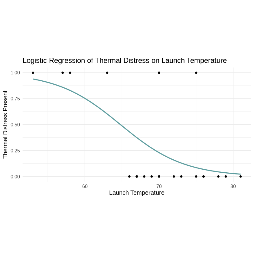
Since the p-value of 0.032 is less than 0.05, we can reject the null hypothesis and accept the alternative hypothesis. We can conclude that launch temperature is a suitable predictor for our response.

Using ggplot to plot the model over the launch temperature.

# Create the plot
ggplot(df, aes(x = launch_temp, y = if_failure)) +
  geom_point() +
  stat_smooth(method = "glm", method.args = list(family = "binomial"), se = FALSE, col = "cadetblue") +
  labs(
    x = "Launch Temperature",
    y = "Thermal Distress Present",
    title = "Logistic Regression of Thermal Distress on Launch Temperature"
  ) +
  theme_minimal(base_size = 12) +
  theme(
    aspect.ratio=1/2
  )

Odds of an O-ring Failure

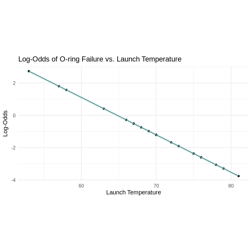
Ploting the log odds over the launch temperature.

predicted_probabilities <- predict(fit, type = "response")
log_odds <- log(predicted_probabilities / (1 - predicted_probabilities)) # logit
plot_data <- data.frame(Temperature = df$launch_temp, LogOdds = log_odds)

# Plot the log-odds against temperature
ggplot(plot_data, aes(x = Temperature, y = LogOdds)) +
  geom_point() +
  geom_smooth(method = "lm", color = "cadetblue") +
  labs(title = "Log-Odds of O-ring Failure vs. Launch Temperature",
       x = "Launch Temperature",
       y = "Log-Odds") +
  theme_minimal(base_size = 12) +
  theme(
    aspect.ratio=1/2
  )

The log-odds decreases with increasing launch temperature. Consider the odds of a lauch with a temperature of $81^\circ$F and another of $80^\circ$F. Take the odds ratio of 81 and 80, we get

As calulated before, $\hat\beta_1$ is aproximately $-0.22$, which means the odds ratio is approximately $0.7928$. This means for every temperature increase of $1^\circ$F the odds of an O-ring failure will change by a factor of $0.79$. In other words as the temperature increases, the odds decreases, as seen in the above figure.

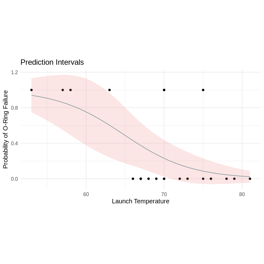
Prediction Intervals

Below is a plot of the model with prediction intervals.

new_temps <- seq(min(df$launch_temp), max(df$launch_temp), length.out = 100)
pred <- predict(fit, newdata = data.frame(launch_temp = new_temps), type = "response", se.fit = TRUE)

# Calculate prediction intervals
upper_bound <- pred$fit + (1.96 * pred$se.fit)
lower_bound <- pred$fit - (1.96 * pred$se.fit)

pred_df <- data.frame(
  launch_temp = new_temps,
  prob = pred$fit,
  upper = upper_bound,
  lower = lower_bound
)

# Add prediction intervals to the plot
ggplot(df, aes(x=launch_temp, y=if_failure)) +
  geom_point() +
  geom_line(data=pred_df, aes(x=launch_temp, y=prob), color = "cadetblue") +
  geom_ribbon(data=pred_df, aes(x=launch_temp, ymin=lower, ymax=upper), alpha=0.2, fill="lightcoral", inherit.aes=FALSE) +
  labs(
    x="Launch Temperature",
    y="Probability of O-Ring Failure",
    title="Prediction Intervals"
  ) +
  theme_minimal(base_size = 12) +
  theme(aspect.ratio = 1/2)

Extrapolating the model

The Challenger launched with a launch temperature of $36^\circ$F in 1986. The smallest temperature in our data is $53^\circ$F. Based on our analysis we can assume the logistic model fit is true. Therefore, we will extrapolate it to this model to this case.

nd <- data.frame(launch_temp = 36)
predict(fit, newdata = nd, type = "response")

The probability estimator of an O-ring failure with a launch temperature of $36^\circ$F is approximately $0.99875$.

Conclusion

In conclusion, the probability of an O-ring failing decreases as the launch temperature increases. In other words, for every 1 degree Fahrenhiet increase in the launch temperature will cause the odds of an O-ring to decrease by $21\%$. Therefore, the likely cause of the Challenger Failure was the cold temperatures as there is an estimated $99.875\%$ probability an O-ring will fail.

In this post, we defined logistic regression and, using the R programming language, applied it to the 1986 Challenger disaster to statistically demonstrate the significance of the Challenger Boosters O-ring failures to launch temperature.