Options trading has become a significant aspect of modern finance, providing traders the ability to hedge risk. The problem of how to fairly price Options is difficult, but can be estimated with the Black-Scholes Model, a mathematical formulation for pricing European Call Options.

In this post we will use Python and the Black-Scholes formula to estimate the fair price of a Netflix Call Option. We will clearly define the formula and assumptions. We will use the yfinance library to fetch Netflix’s historical prices and call options data, and compare the price calculated with Black-Scholes with the price the call option traded at to check if it was a fair price.

What is a Call Option?

Call options are financial contracts that give the buyer the right—but not the obligation—to buy a stock, bond, commodity, or other asset or instrument at a specified price within a specific period.

- Investopedia

The asset is sold at agreed upon price, called the Strike price, and for European Options the date the contract can be exercised is a strict date called the maturity date.

Black-Scholes Formula

The Black-Scholes formula is a mathematical model used to determine a fair non-arbitrage price of a European Call Options contract. We must assume the price of the stock follows a Geometric Brownian Motion, no dividends are paid out and no commission is paid.

Black-Scholes takes the following form

Where

• $C$ is the fair price of the contract
• $S_0$ is the price of this Stock at the time the call option was purchased
• $K$ is the Strike price
• $T$ is the maturity date
• $r$ is the risk free rate
• $\sigma$ is the annual volatility of the Stock
• $\Phi$ is the Cumulative distribution function of a Standard Normal Distribution

The data

Inorder to estimate the price of a Call Option, we need to retrieve Netflix historical stock prices and call option data. To do this we will use the yfinance library.

Retrieving Netflix’s Stock Data

Let’s create a ticker for Netflix NFLX and retrieve the daily historical prices over the last four years.

# Import yfinance library and pyplot module from matplotlib
import yfinance as yf
import matplotlib.pyplot as plt

import datetime
from datetime import timedelta

# Netflix
stock = 'NFLX'
ticker = yf.Ticker(stock)
today = datetime.date.today()

stock_data = ticker.history(
    interval='1d', 
    start=today-timedelta(days=4*365), 
    end=today
    )

# Plotting the closing price `Close` over the last 4 years
stock_data.plot(y='Close'figsize=(12,6))
plt.title(f'{stock} Closing Prices time series')
plt.xlabel('Date')
plt.ylabel('Closing Price')
plt.legend()
plt.show()

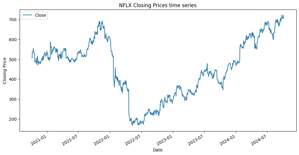
We can use this data to calculate the log-returns of the Netflix stock over four years. Using the pct_change() method from the pandas library, on stock_data will estimate its daily returns. Taking its log will give us the log-returns.

import pandas as pd
import numpy as np

# Returns distributions
daily_returns = stock_data['Close'].pct_change()

# log returns distributions
daily_log_returns = np.log(daily_returns+1)

# Plotting histogram of the log-returns
daily_log_returns.hist(bins=50, figsize=(12,6))
plt.title(f'{stock} Daily Log Returns Distribution')
plt.xlabel('Daily Log Returns')
plt.ylabel('Frequency')
plt.show()

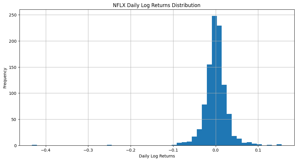
The histogram of log-returns forms a normal distribution. Which verifies our assumption that the stock price must follow a geometric Brownian motion.

The standard deviation of the log-returns times the square root of the number of trading days (252) gives us the annual volatility of the Netflix Stock over the last four years.

The annualised volatility of NFLX is 0.47

Retrieving Netflix’s Options Data

Using yfinance we will retrieve Netflix call option contracts. Choosing an expiry date and a contract to apply to Black-Scholes.

# get all option expirey date
expirations = ticker.options

# Selecting element 7 as the expiry date i.e. 2025-01-17
# list options with a chosen expirey
expiry = expirations[7]

options = ticker.option_chain(date = expiry)

# Get the option with index 2
option = options.calls.iloc[2] 
purchase_date = option.lastTradeDate # Date the Contract was priced
time_to_maturity = pd.Timestamp(expiry + ' 16:00:00', tz='EST') - purchase_date.tz_convert('EST') # The number of days to maturity

Here are some important details on the contract we chose using the above code:

• Contract symbol option.contractSymbol: NFLX250117C00015000
• Last traded purchase_date: 2024-10-04 18:54:09+00:00
• Strike option.strike: $15
• Expiry expiry: 2025-01-17
• Last trading price option.lastPrice: $701.45
• Time to maturity time_to_maturity: 105 days

This contract bought on 4^th October 2024, has a strike price of $15 and has 105 days until the time of maturity (time the contract must be exercised or not).

A key component of the Black-Scholes formula is the price of the stock at the time the contract was purchased. The code below will get the price of the Netflix stock as of the purchase date, 4^th October 2024.

# stock price when option was traded
minute_data = ticker.history(
    interval='1m', 
    start=purchase_date-timedelta(minutes=1), 
    end=purchase_date+timedelta(minutes=5)
    )

# Price of the stock
stock_price = minute_data.iloc[1].Close

print(f'Current stock price: {stock_price:.2f}')

Current stock price: 715.74

Risk Free Rate

It is common to set the risk free rate as the yield on three-month US Treasury-bonds ^IRX. We will use yfinance to retrieve the risk free rate on 4^th October 2024.

# Creating a ticker for `^IRX`
treasury_3m = yf.Ticker('^IRX')

# Risk Free Rate on date the option was purchased (on `purchase_date`)
minute_history_bond = treasury_3m.history(
    interval='1m', 
    start=purchase_date-timedelta(minutes=1), 
    end=purchase_date+timedelta(minutes=5)
    )

# Risk free rate
usbond = minute_history_bond.iloc[0].Close

print(f'Risk Free Rate: {usbond:.2f}%')

Risk Free Rate: 4.51%

The Black-Scholes Formula

Finally, taking the stock price at time of purchasing the call option, strike price, time to maturity, the risk free rate and the volatility of the Netflix stock over the last four years, we can calculate the non-arbitrage (fair) price of the call option.

from scipy.stats import norm

# Black-Scholes Formula
def BlackScholes(S, K, T, r, sigma):
    d1 = ((r + 0.5*sigma**2)*T + np.log(S/K))/(sigma*np.sqrt(T))
    d2 = d1 - sigma*np.sqrt(T)
    C = S*norm.cdf(d1) - K*np.exp(-r*T)*norm.cdf(d2)
    return C

# Fair price of the call option
Call = BlackScholes(
    stock_price, 
    option.strike, 
    time_to_maturity.days/365, 
    usbond/100, 
    volatility
    )

We estimate the Black-Scholes price of the Netflix call option on the 4^th October 2024, to be 700.93. In comparison, the actual market price for the same contract on that date was 701.45. The similarity between the Black-Scholes price and the actual market price reflects how effective the Black-Scholes model is in pricing European Call Options.

Conclusion

In this post we defined and demonstrated the Black-Scholes formula on real world data and used the yfinance library to compare the Black-Scholes price to the actual price of a Netflix call option.