In the early 19th century, physicist Jean Baptiste Joseph Fourier presented in his manuscript “Theorie de la Propagation de la Chaleur dans les Solides”, the Heat Equation. The Heat Equation, describes the flow of heat through solids. It is a Partial Differential Equation and takes the following form,
\[\frac{\partial u}{\partial t} = D\nabla^2u,\]where $u(\mathbf{x}, t)$ is the temperature and a point $\mathbf{x}$ and at time $t$, and $D$ describes the rate of heat transfer through the solid.
This post is split into two main parts:
- Deriving the Heat Equation in three dimensions
- Solving it in one dimension and applying the solution to a one dimensional rod
Part 1: Derivation
Consider a 3 dimension region $\Omega \subset \mathbb{R}^3$ with surface boundary $S = \partial \Omega$. We are interested in looking at the heat flow or thermal flux through this region. We will denote the flux as $\mathbf{q}(\mathbf{x}, t)$ where $\mathbf{x} \in \Omega$ and $t \geq 0$. The flux can be represented a vector field. All the sinks or sources inside $\Omega$ will cancel out. Therefore, the overall flux in $\Omega\setminus S$ is $0$. So we can use the Divergence Theorem:
\[\iiint_\Omega \nabla \cdot \mathbf{q}dV = \Large{\text{∯}}_{\small \partial\Omega} \normalsize \mathbf{q}\cdot d\mathbf{S}\]Let $u(\mathbf{x}, t)$ is the temperature at the point $\mathbf{x} \in \Omega$ and time $t$. Fourier’s law says the flux is proportional to negative the spatial change in temperature. In three dimensions, this can be described using the gradient operator $\nabla$,
\[\mathbf{q} = -k\nabla u\]The proportionality constant $k$ is known as the thermal conductivity of the region $\Omega$.
The internal energy (heat energy) is given by the formula $dQ = \sigma u dm$, over an infinitesimal mass $dm$ with temperature $u$ and specific heat capacity $\sigma$. For the purposes of this problem we will rewrite the mass in terms of an infinitesimal volume of $\Omega$, using the density $\rho = \frac{dm}{dV}$. Now we can express the infinitesimal heat as $dQ = \rho\sigma u dV$. The total internal energy $Q$ is written as,
\[Q = \iiint_{\Omega} \rho\sigma u dV\]By the conservation of energy the rate of change of the heat should be the same of the thermal flow through the boundary $S$. Therefore,
\[-\frac{dQ}{dt} = \Large{\text{∯}}_{\small \partial\Omega} \normalsize \mathbf{q}\cdot d\mathbf{S}.\]Combining everything we discussed together, we get this,
\[\iiint_{\Omega} \nabla\cdot(-k\nabla u)dV = - \frac{d}{dt}\iiint_{\Omega}\rho\sigma u dV.\]For simplicity, we will assume $k$, $\rho$ and $\sigma$ can come outside the integral. The derivative can go inside the integral sign and become a partial derivative.
\[\begin{equation}k\iiint_{\Omega} \nabla\cdot(\nabla u)dV = \rho\sigma\iiint_{\Omega} \frac{\partial u}{\partial t} dV,\end{equation}\]and $\nabla \cdot (\nabla u) = \nabla^2 u$ which is called the laplace Operator, and is defined as,
\[\nabla^2u = \frac{\partial^2 u}{\partial^2 x} + \frac{\partial^2 u}{\partial^2 y} + \frac{\partial^2 u}{\partial^2 z}, (x, y, z) \in \mathbb{R}^3.\]Therefore, we can now say,
\[\frac{k}{\rho\sigma}\iiint_{\Omega} \nabla^2udV = \iiint_{\Omega} \frac{\partial u}{\partial t} dV.\]Since both sides are integrated over the same domain, we can take out the integrand expressions and set them equal to get,
\[\frac{\partial u}{\partial t} = D\nabla^2u\]where $D = \frac{k}{\rho\sigma}$.
We have derived the Heat Equation. Now let’s solve it!
Part 2: Solving the One Dimesional Heat Equation
To simplify this we will solve the heat equation in one dimension. We can think of this as very thin rod with a length of $L$. How does this effect the heat equation? Firstly, we can think of $\Omega$ as the closed interval $[0, L]$ and the boundary as the set ${0, L}$. The Laplace Operator can be written in one dimensional form,
\[\nabla^2u := \frac{\partial^2 u}{\partial x^2}.\]So the adapted Heat Equation is,
\[\frac{\partial u}{\partial t} = D\frac{\partial^2 u}{\partial^2 x}.\]To get a meaningful solution we must introduce initial conditions. Let $u(x, 0) = f(x)$. This can be thought of as the state of our system when time $t$ is zero. We will also need to pick boundary conditions to solve this problem. Let’s define the boundary conditions $u(0, t) = 0$ and $u(L, t) =0$. These are also known as Dirichlet Boundary Conditions.
We will solve this problem by Separation of Variables. We can assume $u(x,t)$ can be written as the product of the time and spatial components. Expressed as,
\[u(x, t) = X(x)T(t)\]Plugging this into the Heat Equation gives,
\[T^{\prime}X = DTX^{\prime\prime}\]Separating the time dependent terms and the spatial dependent terms. If the left-hand side was to change in $t$ then the right-hand side would have to change in $x$ so that is the same as the left-hand side, and vice versa for the right-hand side. So we can say for any value of $x$ and $t$, the two equivalent expressions are constant, which we denote by $-\lambda$ (the minus sign is chosen for convenience). This is written as,
\[\frac{T^{\prime}}{DT} = \frac{X^{\prime\prime}}{X} = -\lambda.\]Separating them, we get the two Ordinary Differential Equations,
\[\begin{align} T^{\prime} + D\lambda T &= 0 \\ X^{\prime\prime} + \lambda X &= 0\end{align}\]We will solve them separately, starting with the equation for $X$, which is also known as Poisson’s Equation.
Solving for $X$
To solve this problem we must take the boundary conditions into account. We will separate $u(0, t) = 0$ and $u(L, t) = 0$ to take the form $X(0)T(t) = 0$ and $X(0)T(t) = 0$. We will neglect the $T$ component, and can express the boundary value problem as follows,
\[\begin{align} X^{\prime\prime} + \lambda X &= 0 \\ X(0) &= 0 \\ X(L) &= 0. \end{align}\]We must consider three cases for $\lambda$ in order to filter out the trivial solutions. Consider Case 1:
Case 1: Let $\lambda = 0$
Then the boundary value problem becomes
\[X^{\prime\prime} = 0\]Solving this gives $X(x) = Ax+B$, where $A$ and $B$ are constants from the integration. Plugging in the boundary values we get the following system
\[\begin{align} X(0) = B &= 0 \\ X(L) = AL+B &= 0\end{align}\]Solving this we get $A = 0$ and $B=0$. Thus, $X(x) = 0$, which leads to the trivial solution $u(x, t) = 0$.
We will neglect Case 1. Now consider Case 2:
Case 2: Let $\lambda < 0$
Then the boundary value problem becomes
\[X^{\prime\prime} - |\lambda|X = 0\]The solution to this Differention Equation takes the form
\[\begin{align} X(x) &= Ae^{\alpha x} + Be^{-\alpha x} \\ &= Ae^{|\lambda|x} + Be^{-|\lambda|x}\end{align}\]Plugging in the boundary values gives the following system
\[\begin{align} X(0) = A+B &=0 \\ X(L) = Ae^{|\lambda|L} + Be^{-|\lambda|L} &= 0\end{align}\]Solving this will also lead to the trivial solution.
We will also neglect Case 2. Consider Case 3:
Case 3: Let $\lambda > 0$
Then the problem has a characteristic polynomial of $\alpha^2 + \lambda = 0$. Therefore, $\alpha = \pm i \sqrt{\lambda}$. The Solution will then take the form:
\[X(x) = A\cos(\sqrt{\lambda} x) + B\sin(\sqrt{\lambda} x).\]Now let’s look at the boundary conditions. Take $X(0) = B = 0$, so we can deduce $B = 0$. Now consider $X(L) = A\sin(\sqrt{\lambda} L) = 0$. We can’t say $A=0$, or we will get the trivial solution, so we need to consider all $\sqrt{\lambda} L$’s such that $\sin(\sqrt{\lambda} L) = 0$. We can say that $\sin(n\pi) =0$ for all positive integers $n$. Therefore, $\sqrt{\lambda} L = n\pi$ or writting $\lambda_n$ as a sequence with index $n$, we can say
\[\lambda_n = \frac{n^2\pi^2}{L^2}.\]
Case 3 gives us a non-trivial solution. Adopting Case 3, we can say a solution to the boundary value problem is,
\[X_n(x) = B_n\sin\left(\frac{n\pi x}{L}\right), n=1,2,3,\dots.\]We can write the full solution as the linear combination of all $X_n(x)$,
\[X(x) = \sum^{\infty}_{n=1} B_n\sin\left(\frac{n\pi x}{L}\right)\]Interesting! This resembles a Fourier Series of an odd function. We must remember back to when we defined the initial condition of our heat system, $u(x,0) = f(x)$. Separating this $X(x)T(0) = f(x)$. Since the time dependent part doesn’t have any $x$ dependencies, we can say $T(0)$ is a constant. Without loss of generality, let’s say that constant is $1$. Now we can say $X(x) = f(x)$. Which means that the above solution is can be thought of as a Fourier series of $f(x)$. Now we can write an expression to define $B_n$,
\[B_n = \frac{1}{L}\int^L_0 f(x) sin\left(\frac{n\pi x}{L}\right)dx.\]Solving for $T$
Solving for $T$ involves less work. Suppose,
\[T^{\prime} + D\lambda T = 0.\]The solution is,
\[T(t) = Ce^{-D\lambda t}.\]Recall, $\lambda_n = \frac{n^2\pi^2}{L^2}$. We can write $T_n(t)$ as,
\[T_n(t) = C_n e^{-D\frac{n^2\pi^2}{L^2}t}.\]We said that $T(0) = 1$ which means $C_n = 1$ for all $n$.
\[\therefore T_n(t) = e^{-D\frac{n^2\pi^2}{L^2}t}, n=1,2,3,\dots\]Now we can combine our solution for $X$ and $T$ to get $u$,
\[u(x, t) = \sum^{\infty}_{n=1} B_n\sin\left(\frac{n\pi x}{L}\right)e^{-D\frac{n^2\pi^2}{L^2}t},\]where,
\[B_n = \frac{1}{L}\int^L_0 f(x) sin\left(\frac{n\pi x}{L}\right)dx.\]Now let’s create an example. Suppose we had a one dimensional rod with length $L=2$, and we set the temperature of the first half of the rod to $0$ and the second to $1$. We can represent the initial condition as,
\[u(x, 0) = \begin{cases} 0 & \text{if } 0 \leq x \leq \frac{L}{2} \\ 1 & \text{if } \frac{L}{2} < x \leq L \end{cases}\]Assuming the coefficient $D = 1$. The solution $u_{\text{rod}}(x, t)$ is expressed as,
\[u_{\text{rod}}(x, t) = \sum^{\infty}_{n=1} \frac{2}{(n\pi)(\cos(\frac{n\pi}{2}) - (-1)^n)}\sin\left(\frac{n\pi x}{L}\right)e^{-D\frac{n^2\pi^2}{L^2}t}.\]The temperature of the rod evolves following the illustration below,
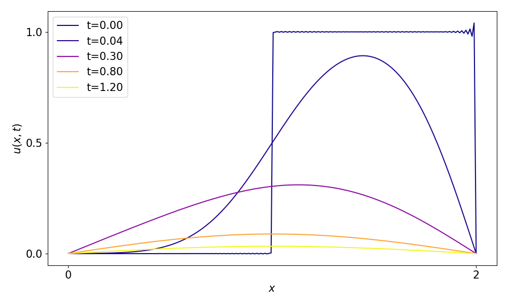
We can see the temperature of the rod smoothens out over time, becoming more and more homogeneous. This phenomena is called Diffusion, and a more general name for the heat equation is the Diffusion Equation.
Now we have “a solution”. I put emphasis on “a solution” because it is not the only kind of solution. This is a solution in one dimension with finite boundary conditions. There are solutions for the Heat Equation where we define the temperature over the entire real line $\mathbb{R}$, we could call these infinite boundaries. There are also semi-infinite boundary conditions which are solutions defined over the interval $[0, \infty)$. To approach we would need to use Fourier Transforms.
We can also consider a finite boundary value problem where instead of zero temperature on the boundary the flux, $-\nabla u$ is zero. This type of problem is known as a Neumann Boundary Value Problem.
Further Exploration
Numerical Methods such as the Finite Difference Method can also be applied to solve this problem. Have a look here to see a brief overview of this.
We mentioned that the Heat Equation is also known as the Diffusion Equation. The Diffusion Equation can be appears in many areas such as: Finance, Biology, Fluid Dynamics and Physics. It had a profound impact on mathematical modelling and shaped much of how we understand dynamic processes.